
Digging into Deviations in the Cast Vote Record
Election researchers have extensively used cast vote record (CVR) analysis to alert the public to deficiencies in our local, state, and national elections.
Election and CVR Basics
A CVR is an electronic record of the choices made on a ballot. The term is also often used to refer to the aggregation of all such records for a single election, and it is the latter definition that I will use throughout.
CVRs matter because auditing matters. We have no reason to be confident in the outcome of an election if we cannot also have confidence in the process steps and data that led to that outcome. The abundant data in a CVR provide us the ability to run many types of statistical analysis in our search for clues to deviations from expectations.
A good and proper election can be defined as: “An election in which the officially reported results accurately reflect the informed will of all legitimate and only legitimate voters.”
The obvious requirements of this definition have many subsidiary requirements. Failure of a single requirement is sufficient to compromise an election. Failure of multiple requirements is catastrophic.
The requirements may fail due to human or machine error, legislative incompetence, or to nefarious activity. It’s critical to understand the types of nefarious activity that might affect our elections. I categorize fraud into three types:
Voter fraud – When an individual or a small group casts ballots to which they are not entitled.
Election fraud – An organized, well-resourced effort to swing a contest in one election by one or a combination of methods.
Systemic fraud – An organized, well-resourced effort to hijack an entire election system. This is potentially permanent, and is pervasive across contests, time, and locale.
We often hear about voter fraud, and occasionally about election fraud. Systemic fraud by its very nature would not be widely known or publicized. Statistical deviations such as those identified in CVRs should be considered in the context of potential election or systemic fraud.
Statistics rarely prove a matter, because the numbers themselves aren’t a crime. At best, one can conclude beyond a reasonable doubt that a crime occurred, but the challenge becomes one of finding the evidence that caused the unusual statistics or deviations.
Some of the metrics often used in CVR analysis include: cumulative ratio (CR), sliding block ratio, and linked contests (like Solomon, below).
The CR is intended to give a high-level picture of the entire election to determine if it approximates expectations. This ratio is based on the Law of Large Numbers (LLN), which states the expectation that a large number of independent trials (votes, coin flips, etc.) can be approximated by a much smaller number of trials. Genuine polling uses this principle to estimate the choice of a large population by asking a much smaller population. According to the AI tool Grok the LLN is based on three assumptions:
Votes are cast independently
Voter preferences follow a consistent distribution
The cast vote record reflects the true vote count, without systematic biases or errors
The Sliding Block Ratio is very similar to a moving average in the stock market. Each measurement represents the ratio of candidate A to candidate B in the previous N (typically 500) ballots. This metric is finer-grained than CR.
Case Studies: A Comparison
I’ve reviewed CVRs from hundreds of counties across the country, to varying degrees of detail. I present some of my own research experiences as well as some key findings by other researchers.
Below in Figure 1 is a simulated result of a close election in which the winner obtained 52% of the vote. The final value of the ratio is 1.08. Unsurprisingly this ratio converges to its ultimate value after fewer than 10% total votes have been counted and maintains that value for the remainder of the election. This chart represents our model based on the LLN assumptions noted above.

Fig. 1 Simulated Cumulative Ratio
Twice I have presented cast vote record analysis to election officials. I received substantially similar responses from both officials, namely that “that’s how voters vote”. I was puzzled the first time this happened, because I expected the official to be alarmed by what I presented to him. By the time I spoke with the second official I realized that these officials did not conceive that an election CR should roughly follow the LLN. Divergence when we should expect convergence raised no concerns because they had no expectations.
Following are the combined CR and block ratio charts from San Benito County CA and Yamhill County OR. In all charts the solid line (usually orange) represents the CR of the candidates as the ballots were counted, while the dotted line (usually blue) represents the candidate ratio of the previous 500 ballots. The x-axis is the percentage or fraction of ballots counted.
The two charts are strikingly different. Early during the counting Yamhill County shows its strongest preference for Biden, including a drop and a bounce, before declining regularly until the final votes are counted. San Benito County, on the other hand, begins at a moderate level relative to the final count, then drops slightly before rapidly ascending to a peak at around 32% of the final count. Following the peak we note a chaotic decline until approximately 62% of the votes have been counted, after which the decline is essentially uniform until the conclusion of counting.

Fig. 2 San Benito County Cumulative and Block Ratios
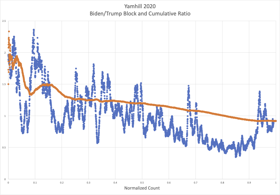
Fig. 3 Yamhill County Cumulative and Block Ratios
Neither county even remotely approaches the simulated result shown earlier. Are these deviations natural? The result of human or machine error? Of malicious code or remote manipulation? Having examined the charts of other counties near both San Benito and Yamhill counties I found no charts that were substantially like either of them. However, San Benito bears surprising similarity to Coos County OR in several respects.
San Benito and Coos County demographics could not be more disparate. Race, religion, occupation, urban/rural concentrations, and party affiliation are highly dissimilar. The tally results are unsurprisingly diverse, but the forms of both Cumulative and Block Ratio plots are strikingly similar between the counties, even though these forms are rarities among all the charts I have seen. A trained eye will note that the volatility of block ratios suddenly declines near the 62% completion mark. The rise and fall of CR represents a change in voter character over time, first in one direction then in the other. How could such things occur naturally in both counties? How could the CR ramp aggressively at the start before concluding gracefully in both plots? Some researchers (see Draza Smith: https://electionfraud20.org/draza-reports/) suggest that the graceful declines in these charts have the appearance of a software-controlled system with a predetermined setpoint.
Elections are not expected to match the model perfectly, but most votes are believed to be cast independently in both counties. Voter preferences could vary, given news cycles and emotional intensity, and may even realistically be expected to vary perceptibly, but it is difficult to believe that variation in voter preference could account for the difference in observed magnitudes. We are left with serious questions about the third assumption of LLN, that the CVR reflects the true vote count without systematic errors or bias. Some critics have argued against application of LLN to elections, as the great majority of CVRs collected from 2020 and since differ meaningfully from the simulation. It is worth noting here that of over 800 CVRs from 28 states only a handful matched the model. That some did match could be the exception that proves the rule.

Fig. 4: San Benito County and Coos County Block Ratio

Fig. 5: San Benito County and Coos County Cumulative Ratio
While the above discussion argues for heightened concern and investigation of our election system it does not represent proof of compromised systems. Proof requires multiple reference points.
Case Studies: Mesa County CO and Shasta County CA
Among the investigations that can possibly explain the observed statistical deviation is one that occurred in Mesa County CO. A second set of database tables were created on the election management server with the net effect being the apparent elimination of some legitimate ballots and possible modification of others, effectively a preloading of preferred ballots. Such preloading could explain the frequent observation of an early lead by candidates who are “preferred” by a malicious intruder. If true, then Mesa County may be only one among many counties in which this malicious action took place. A post-election audit would easily miss an intrusion such as what occurred in Mesa County, because eliminated ballots wouldn’t appear in the CVR, from which the post-election ballots are selected. With a similar but less dramatic theme, in Shasta County in March of 2024, 100 ballots that were scanned and adjudicated never appeared in the CVR and would not have been selected for audit. While I have always expected to find a non-nefarious explanation for these “missing” 100 ballots, the Shasta Elections office has been aware of this concern for nearly a year with no explanation, even though a county supervisor contest was decided by 14 votes.
Case Study: Hart Intercivic CVRs
Most vendors produce(d) CVRs in a spreadsheet-compatible format that easily imports into Excel. Hart Intercivic, however, customarily delivers its CVRs as a zip file containing thousands of xml files, one xml file per ballot. Most intrepid researchers who examine CVRs would be stymied by a Hart CVR because there is no way to import it into Excel or any other spreadsheet. It takes programming skills to convert the xml files into spreadsheet-ready files. While not denying public access to CVRs the Hart systems still exhibited lack of transparency by making the CVRs useless to most researchers.
The xml files have a timestamp. Most timestamps are consistent with the known ballot processing dates during an election. However, when looking at Nevada County, Humboldt County, Solano County, and the state of Hawaii (among others) we find xml file timestamps on January 1 of the year in which the election took place. This precedes ballot mailing for both primary and general elections! We have found an exact match in most counties between the in-person ballots and the xml files with January 1 timestamps. In a few other counties there is a near match. This is problematic, because the timestamp is either meaningless or it means something that it should not.
The election officials I have asked cannot explain the reason for the early timestamp. They refer me to the vendor. Vendors are private companies not subject to public information requests.
Case Study: Linked Contests
Finally, I would mention mathematician Ed Solomon’s work on Arapahoe County from the 2020 election. In Arapahoe county, when across the state of Colorado Republicans voted 65-70% against Measure B (a tax increase) and Democrats voted 30-33% against it, 43% of both Republicans and Democrats voted against the measure. The CR of Trump votes to No votes, compared to the ratio of Biden votes to No votes, is a near-perfect match. The way Republican and Democrat voters reached their final total of 43% “No” cannot occur naturally, nor is it likely to occur through human or machine error. This leaves election interference as the likely explanation.

Fig. 6: Arapahoe County Republican and Democrat Percentage Voting No on B
Challenges
Those with nothing to hide hide nothing. Many election officials have been hesitant to provide election records, and increasingly those records that are provided are difficult to use or have important information redacted. Our current Secretary of State has consistently acted toward restricting access or utility of such documents. At a time when many voters (of all persuasions) have concerns about the outcome of our elections we need greater transparency, not less.
As with any complex business the final metrics used to determine profit or loss, or winners and losers, is subject to potential manipulation. Auditability is essential for those invested in an operation to have confidence in the legitimacy of the outcome. Statistical analysis of CVRs is one method of election auditing that can expose errors or manipulation. Many CVR studies (e.g., Solomon and Arapahoe County) have demonstrated that innocent explanations of the data are unlikely. It is incumbent upon election officials and law enforcement to investigate and determine the physical and electronic means by which the deviations occur. The means may include programmatic activity on the electronic voting system, or any of hundreds of other methods by which elections can be compromised. The consequences of inaction are grave.